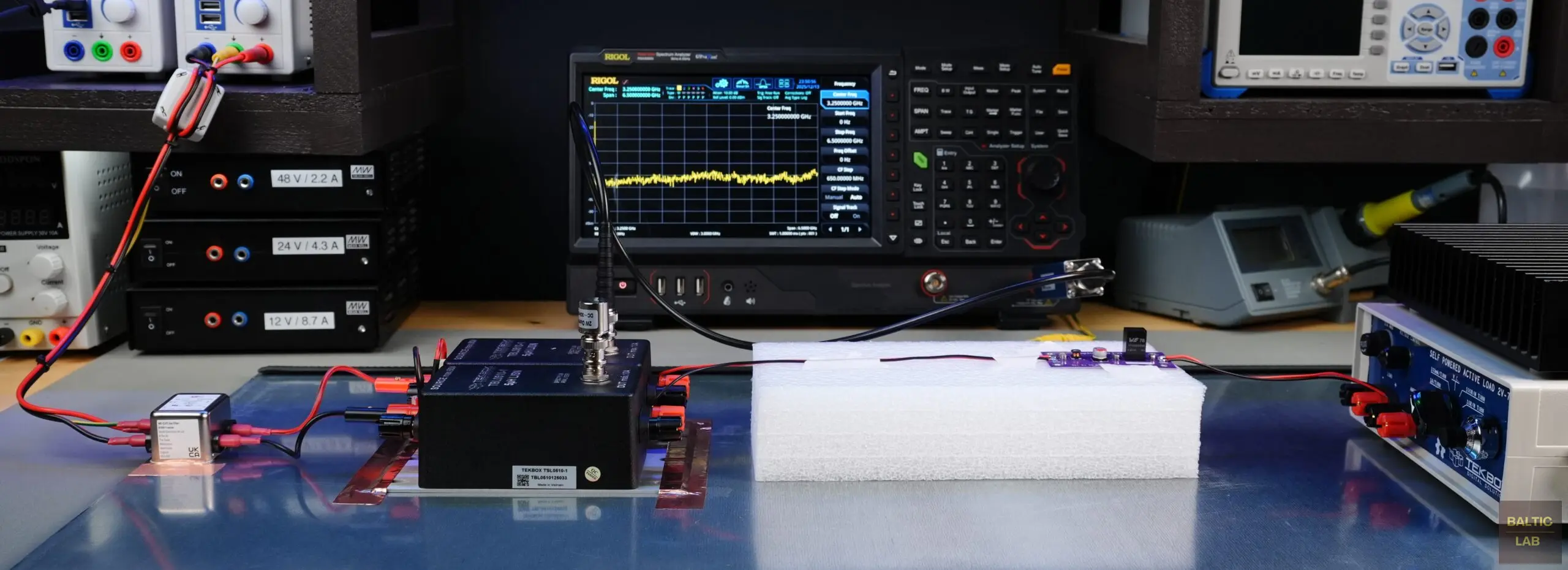
Figure 1: Overview of the benchtop CISPR 25 conducted emissions (voltage method) test setup
Introduction
Electromagnetic compatibility (EMC) is an often overlooked and somewhat enigmatic area of electronics engineering. Its mystique primarily arises from the numerous standards that are not freely accessible and the undeniable gatekeeping of the small professional EMC community. Moreover, EMC test equipment can be prohibitively expensive, discouraging hobbyists and semi-professionals from hands-on experimentation and limiting opportunities to gain practical experience in this critical field. By presenting this relatively low-cost test setup and highlighting the intricate details and requirements dictated by the standard, I aim to lower the barrier of entry for those exploring EMC testing for the first time. At the same time, the setup remains as close to standard-compliant as possible, with all deviations clearly outlined to meet the needs of professional users as well.
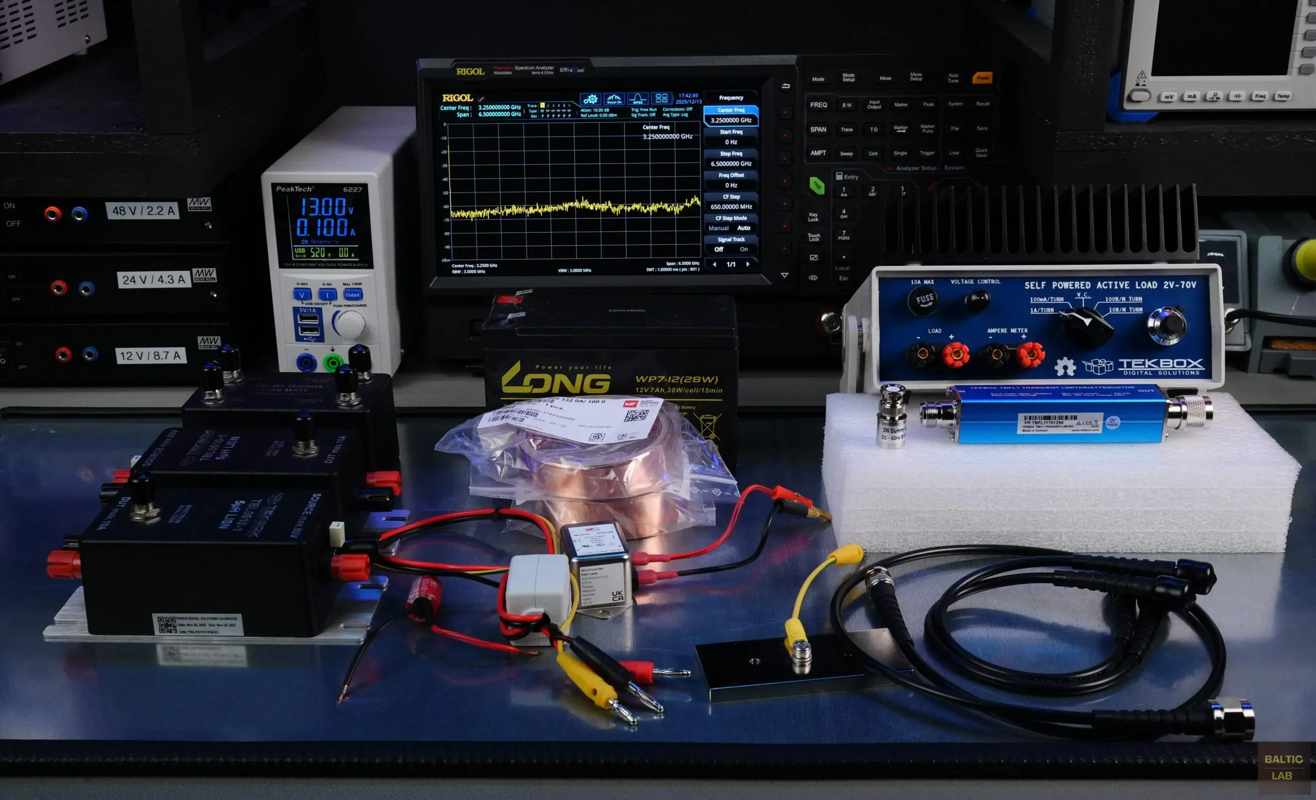
Figure 2: All equipment and accessories required for a largely standard-compliant CISPR 25 (voltage method) test setup
CISPR 25 applies to electronic and electrical components intended for use in vehicles, boats, and devices powered by internal combustion engines. The standard is designed to provide protection for sensitive radio receivers against on-board radio frequency (RF) emissions in the range of 150 kHz to 108 MHz [1].
While CISPR 25 defines limits and test methods for both conducted and radiated emissions, this article focuses exclusively on conducted emissions. For these, the standard provides two measurement approaches: the voltage method and the current method. The setup presented here is based on the voltage method, which is the most space-efficient option. Importantly, the voltage method is also the approach used in accredited compliance laboratories and forms the basis for conducted emissions measurements with an RF current probe, as well as radiated emissions measurements under the same standard. These variants mainly differ in minor details, such as the minimum size requirements for the reference ground plane.
Reference Ground Plane
For conducted emissions measurements using the voltage method, the reference ground plane should be at least 100 cm × 40 cm and made from copper, brass, bronze, or galvanized steel, with a minimum thickness of 0.5 mm [1]. In my setup, I use a 100 cm × 40 cm sheet of galvanized steel with a thickness of 2 mm. Two 1 m sections of rubber edge protection are added to shield against the sharp edges and corners of the steel plate. Deburring would work as well, but it doesn’t look nearly as neat.
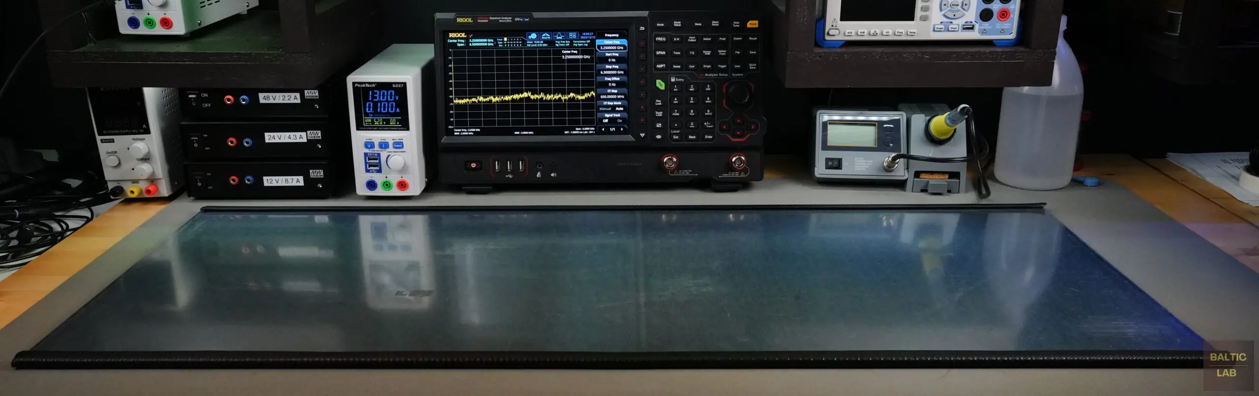
Figure 3: 100 cm × 40 cm galvanized steel sheet, 2 mm thick, used as the reference ground plane
As a useful side note: The minimum ground-plane size for conducted emissions measurements using the current method is 250 cm × 40 cm, and for radiated emissions measurements it is 100 cm × 200 cm. If you plan to perform those tests as well, it may be sensible to invest directly in a properly sized ground plane, and a larger bench. 🙂
The reference ground plane should be positioned at a height of 90 cm ± 10 cm above the floor. My bench has a height of 85 cm, which lies well within the range specified by the standard.
According to the standard, measurements must be conducted in an anechoic chamber or in a shielded room [1]. This requirement conflicts with a truly benchtop pre-compliance setup and is therefore not implemented in my configuration. While skipping a fully shielded environment simplifies the setup, it can increase background noise and external interference, potentially affecting measurement accuracy. Therefore, a background scan should be performed prior to testing to ensure that any external interference is at least 6 dB below the desired limit.
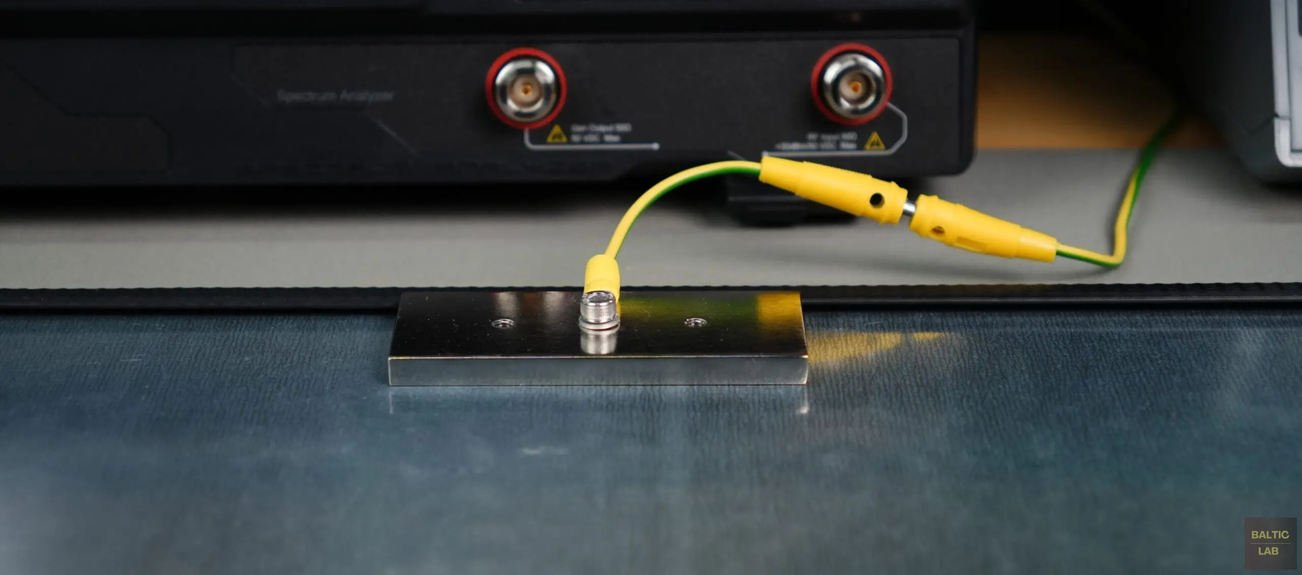
Figure 4: Reference ground plane bonded to earth ground
Ordinarily, the reference ground plane would be bonded to the shielded room, with ground straps spaced no more than 30 cm apart. In addition, each strap must maintain a length-to-width ratio no greater than 7:1 [1]. Due to the lack of a suitable shielded room to bond to, this requirement is also not fully implemented. Instead, a single 6 mm² grounding wire is used. While this simplified grounding approach is sufficient for pre-compliance testing, it may slightly affect repeatability and introduce small measurement variations compared to a fully compliant setup.
Line Impedance Stabilization Network (LISN) / Artificial Network (AN)
A Line Impedance Stabilization Network (LISN), referred to as an Artificial Network (AN) in CISPR standards, is a critical component in conducted emissions testing. Its main purpose is to provide a defined impedance between the power supply and the device under test (DUT) while isolating the DUT from external noise on the supply lines. This allows for repeatable and accurate measurement of RF emissions generated by the DUT. Additionally, the LISN directs electrical noise generated by the DUT to a 50 Ω RF output, suitable for connection to a spectrum analyzer or measurement receiver.
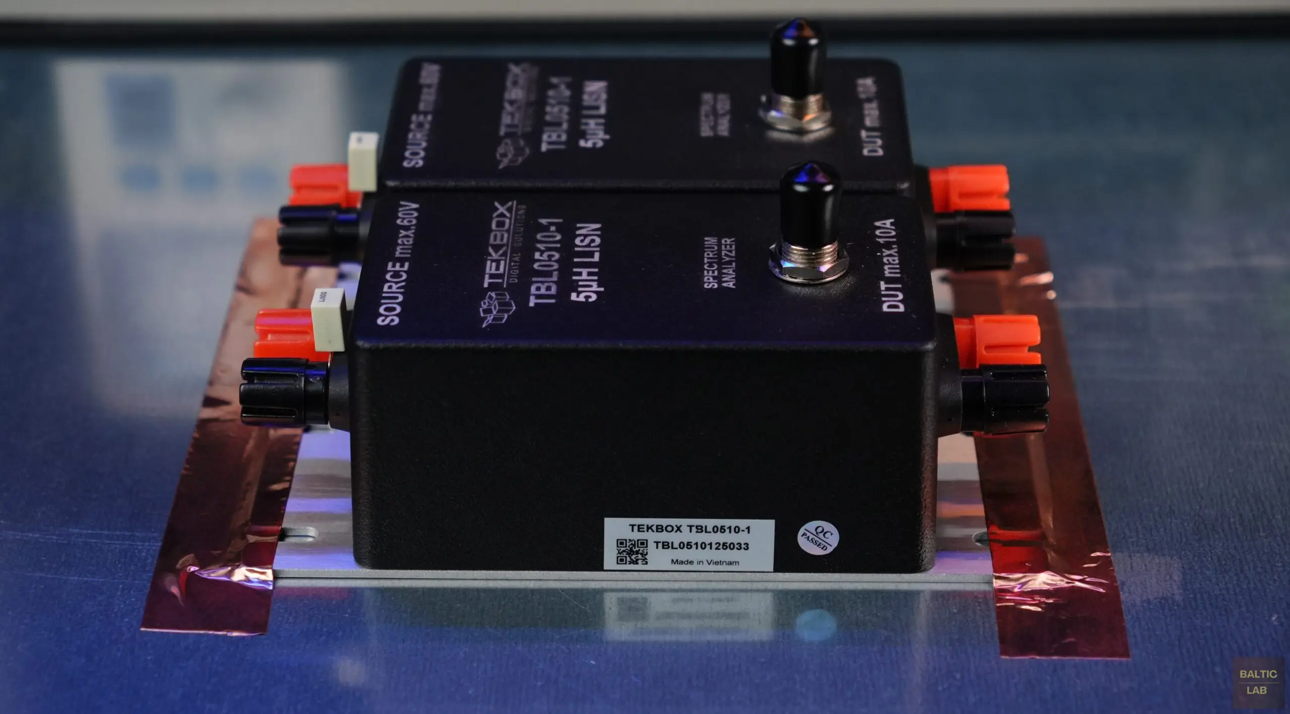
Figure 5: Two TekBox TBL0510-1 5 µH LISNs securely bonded to the reference ground plane using copper tape strips; the factory-installed 1 µF capacitor on the ground-return LISN (right) has not yet been removed
For CISPR 25 conducted emissions measurements, the LISN must have a nominal inductance of 5 µH, exhibit the impedance profile specified by the standard, and be mounted directly on the reference ground plane with its housing electrically bonded to the plane. In my setup, I am using two low-cost TekBox TBL0510-1 LISNs [4]. These LISNs meet the stringent requirements of the standard for impedance profile, impedance phase angle, and isolation. They are also compliant with additional standards such as MIL-STD-461F, DO-160 (Avionics), NATO AECTP-500, and ISO 7637-2, making them highly versatile for use in a variety of test setups.
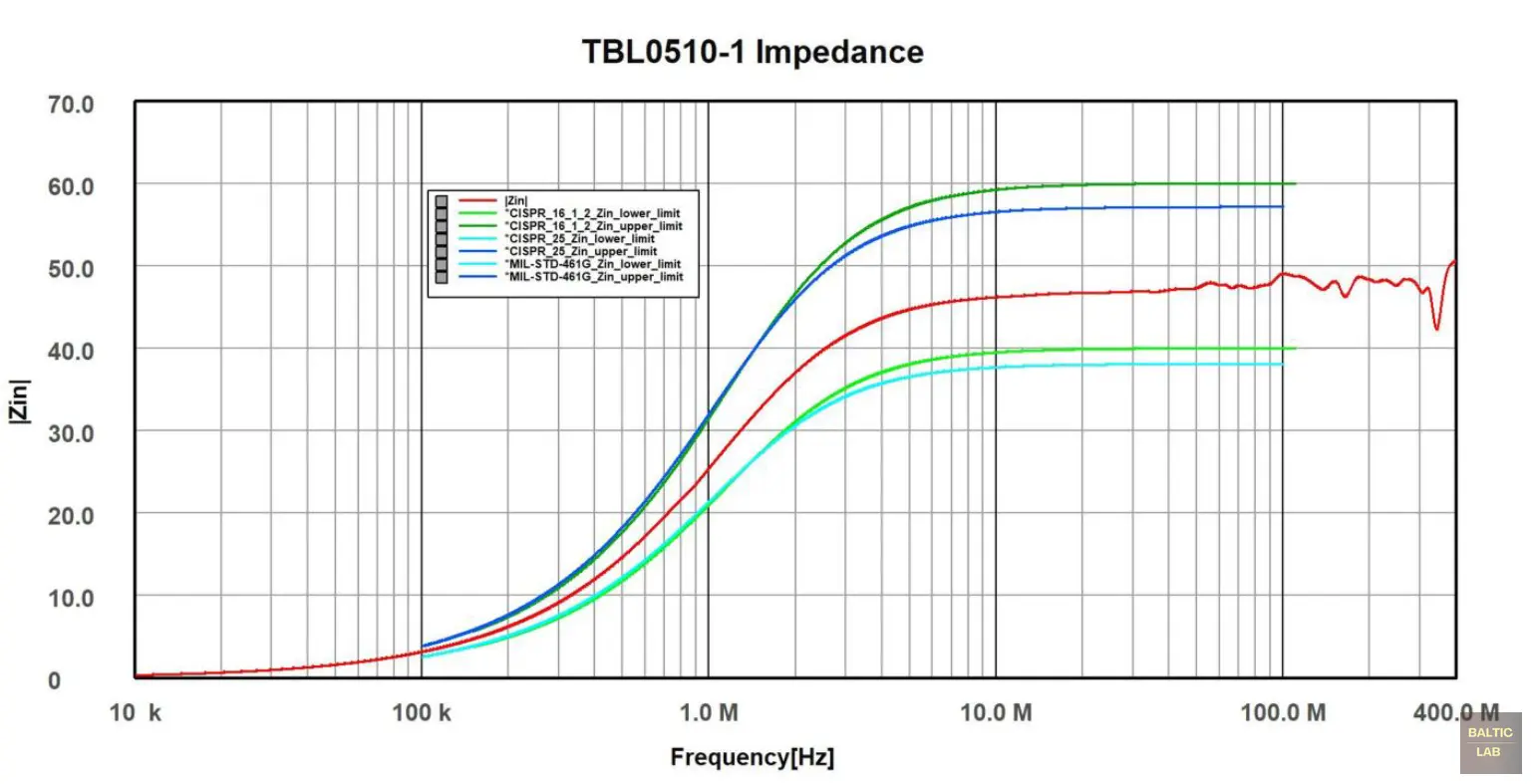
Figure 6: Measured impedance of the TBL0510-1 5μH LISN, 100 kHz – 110 MHz, source terminals shorted [3]
The number of LISNs required depends on both the DUT and the length of its supply cables. For a DUT with a single positive supply and ground, and a supply cable of 20 cm or less, a single LISN is sufficient (Fig. 7). In this case, the DUT’s ground return is directly connected to the reference ground plane, a configuration referred to in the standard as a “locally grounded” DUT.
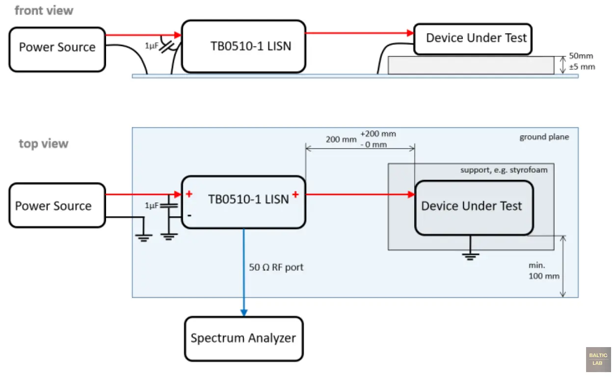
Figure 7: Conducted emission measurement, voltage method, DUT with power return line locally grounded [3]
A more common setup, however, is the “remotely grounded” variant, where both the positive supply line and the ground return are routed through separate LISNs (Fig. 8). The dual-LISN setup also offers the advantage of separating differential- and common-mode noise for troubleshooting. More on that later.
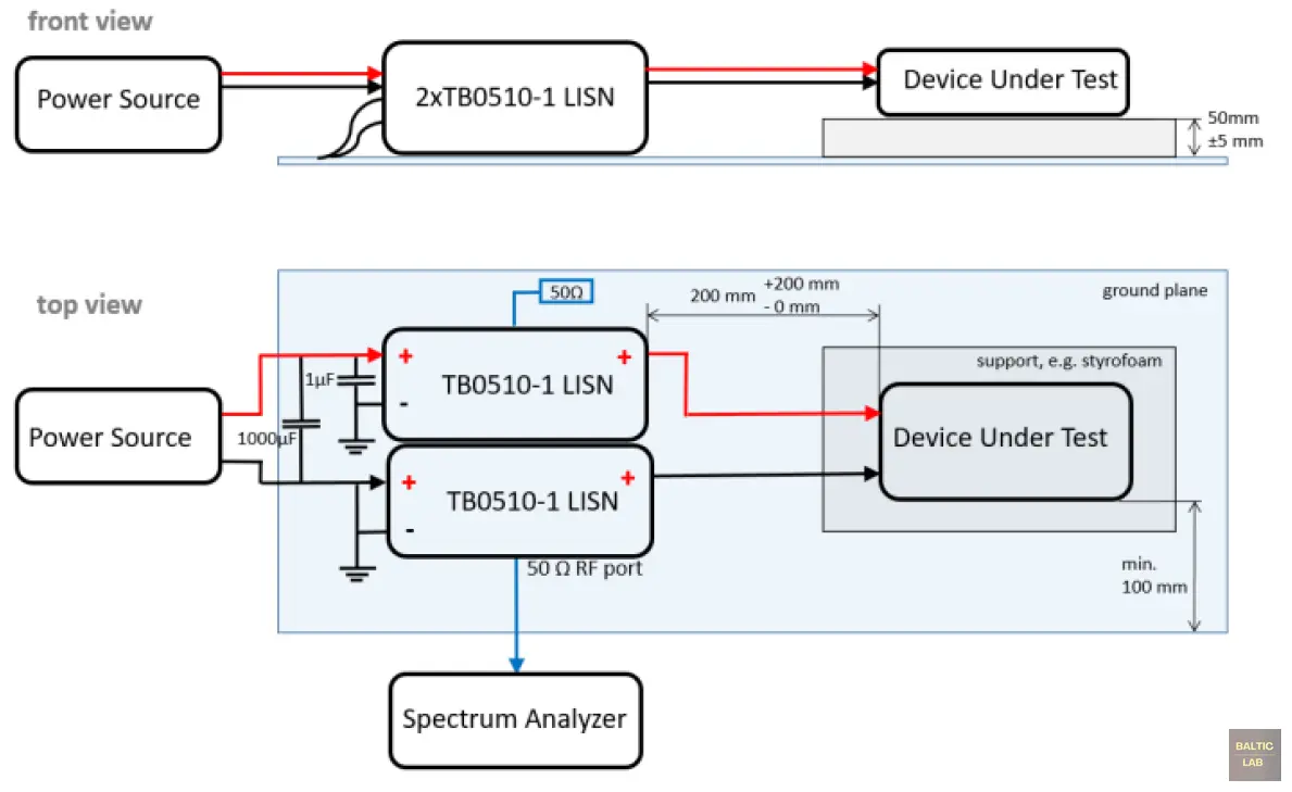
Figure 8: Conducted emission measurement, voltage method, DUT with power return line remotely grounded [3]
A 1 µF capacitor must be connected in parallel at the LISN’s source terminal in the positive supply line (Fig. 8). In the new TBL0510-1 units used here, this capacitor is already included in both characterization and packaging. For the previously used, now end-of-life TBOH01, it must be sourced separately. An additional 1000 µF capacitor must be placed between the positive input terminals of both LISNs (Fig. 9). A Würth Elektronik WCAP-ATG8 rated for up to 63 V is used in my setup [13]. Whether external capacitors must be added to the test setup depends on the LISN manufacturer; some integrate them, others do not. This naturally raises the question of why a required component would be omitted. The answer is not cost-cutting, but functionality: This allows the LISNs to be used more flexibly across different standards. For transient testing under ISO 7637-2, for example, the 1 µF capacitor can simply be removed. For conducted emissions testing of aviation equipment under DO-160, a 10 µF capacitor can be installed in place of the 1 µF cap.
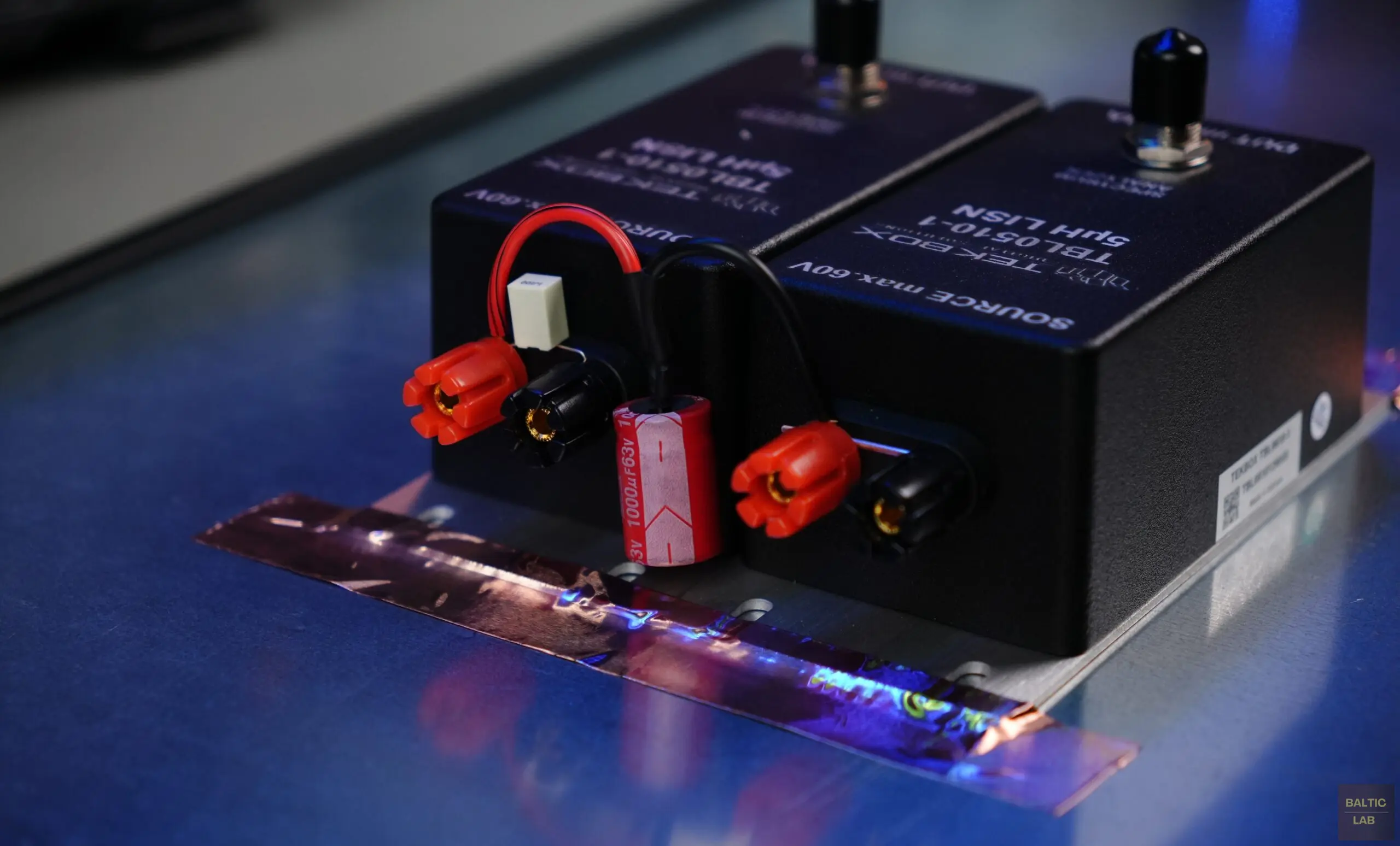
Figure 9: LISNs with a factory-installed 1 µF capacitor on the positive supply line LISN (left) and an externally installed 1000 µF capacitor on the ground-return LISN (right)
Supply Line Routing and Support
The device under test must be positioned on a support made of non-conductive material with a relative permittivity of εr ≤ 1.4, at a height of 50 mm ± 5 mm above the reference ground plane. The supply lines must be routed in a straight line on a similar low-permittivity support at the same height. All sides of the device under test must be at least 100 mm from the edges of the reference ground plane. The power supply’s ground return must also connect to the reference ground plane between the supply and the LISN.
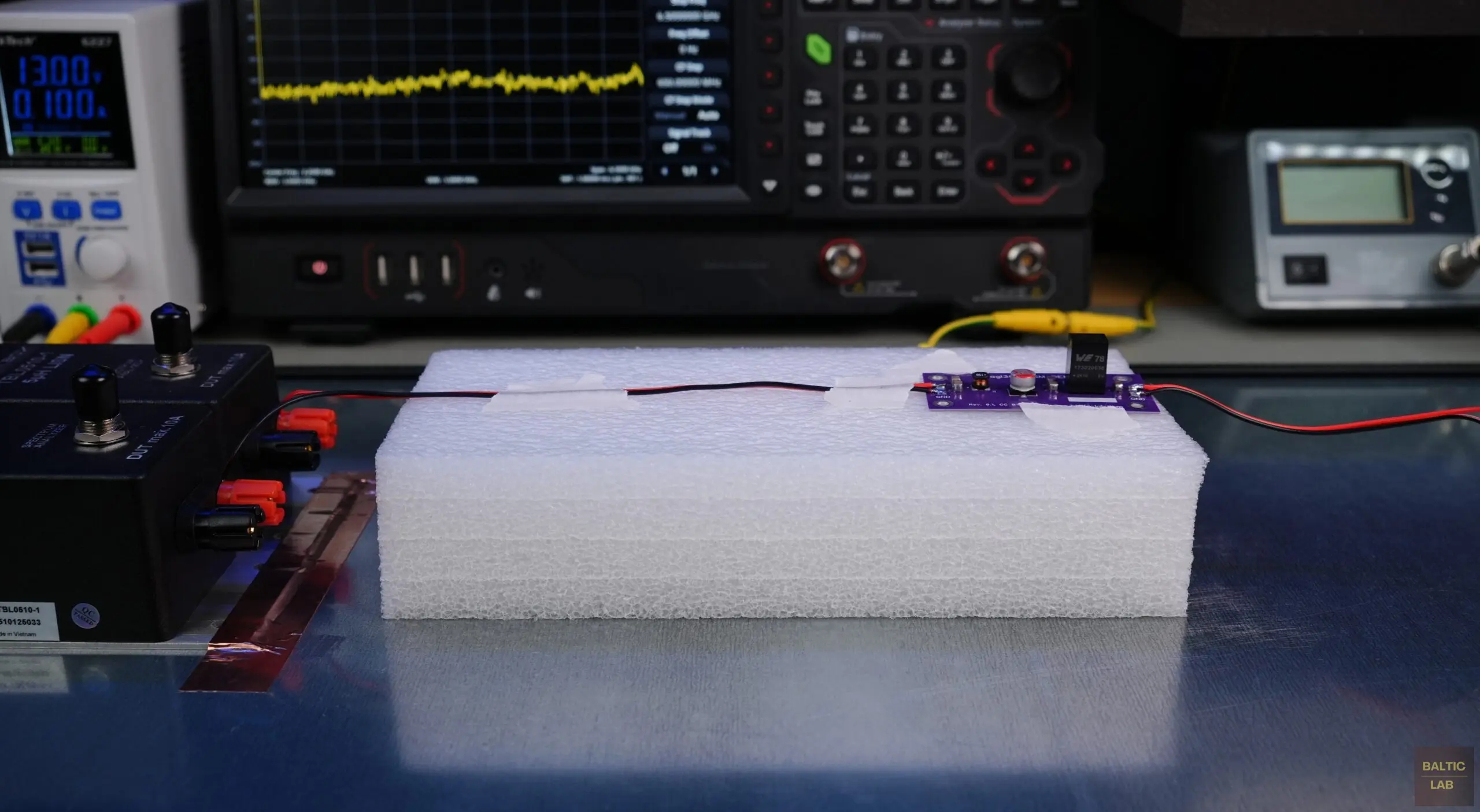
Figure 10: Supply lines and DUT mounted on a low-permittivity support
ESD foam, also known as anti-static foam, is unsuitable as a support because of its conductivity. In my setup, I use 50 mm polyethylene (PE) protective foam. Attentive readers may notice that bulk PE has a relative permittivity of about 2.25, exceeding the permissible εr ≤ 1.4. However, the high air content of PE foam reduces its effective εr to roughly 1.6, still slightly above the limit. A better choice would be styrofoam (expanded polystyrene), which typically has an εr only slightly above 1.
Load Simulator
If the DUT is a stand-alone device that only requires power and has no other external connections, this chapter can be skipped. Otherwise, a load must be included in the test setup, and all actuator and sensor connections normally interfacing with the DUT should be present during measurement. For a simple load, this can often be achieved with a fixed resistor, while a more versatile solution is an active load. While “load simulator” may sound excessive for simple setups, it is the terminology used in the standard.
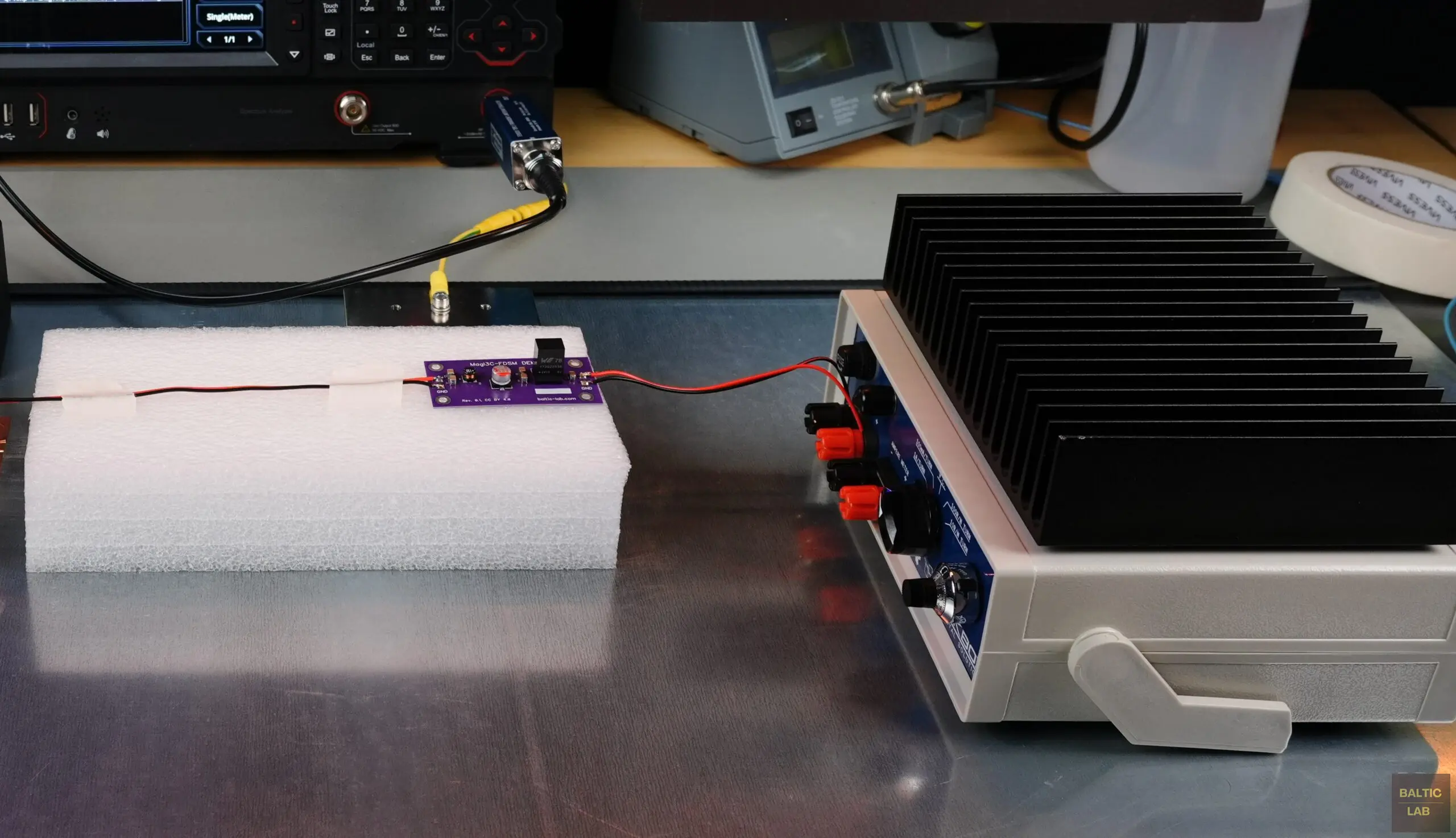
Figure 11: Self-powered active load configured as load simulator and connected to the DUT
The load simulator includes sensors and actuators and terminates the harness connected to the device under test [1]. It should preferably be placed directly on the reference ground plane. If the simulator has a metal housing, the housing must be electrically bonded to the ground plane. Alternatively, it can be positioned in close proximity to the reference ground plane, provided the housing is electrically bonded, or even outside the measurement chamber, as long as the DUT’s harness passes through an RF barrier and remains electrically bonded to the reference ground plane [2]. If the load simulator requires its own power supply, it is important that its DC supply lines are connected directly to the power source and not routed through the LISNs.
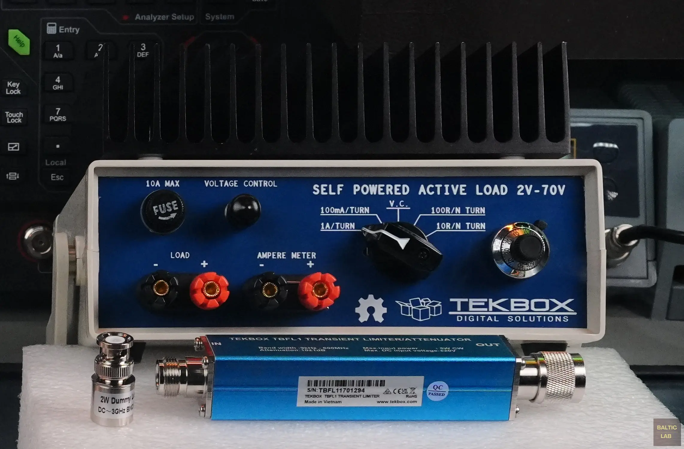
Figure 12: TekBox TBOH02 self-powered active load used as a load simulator
For my setup, a TekBox TBOH02 self-powered active load is used. It requires no external supply, operates from 2 V to 70 V, can sink up to 10 A and supports both constant-current and constant-resistance modes. A 10-turn potentiometer with dial, a range switch, and a precision reference allow accurate setting, and the fully analog design avoids introducing digital noise into supply-noise measurements [10].
Power Supply
The standard sets strict requirements for the power supply. During testing, the DC output must be held at its nominal value ±10%, and the supply must be filtered well enough that any RF noise it produces remains at least 6 dB below the applicable limit. Meeting this condition can be challenging even for well-regulated switch-mode supplies.
| Nominal Supply Voltage | Test Voltage |
|---|---|
| 12 V | 13 V ± 1 V |
| 24 V | 26 V ± 2 V |
| 48 V | 48 V ± 4 V |
While a linear supply is generally preferred, I use a PeakTech 6227 0-60 V switch-mode supply together with additional filtering to ensure the required 6 dB margin below the CISPR 25 Class 3 limits. A Würth Elektronik WE-CLFS single-stage line filter [8] together with a WE-STAR-TEC snap-on ferrite [9] is used to filter the connection between the power supply output and the LISN input. The line filter is bonded directly to the reference ground plane.
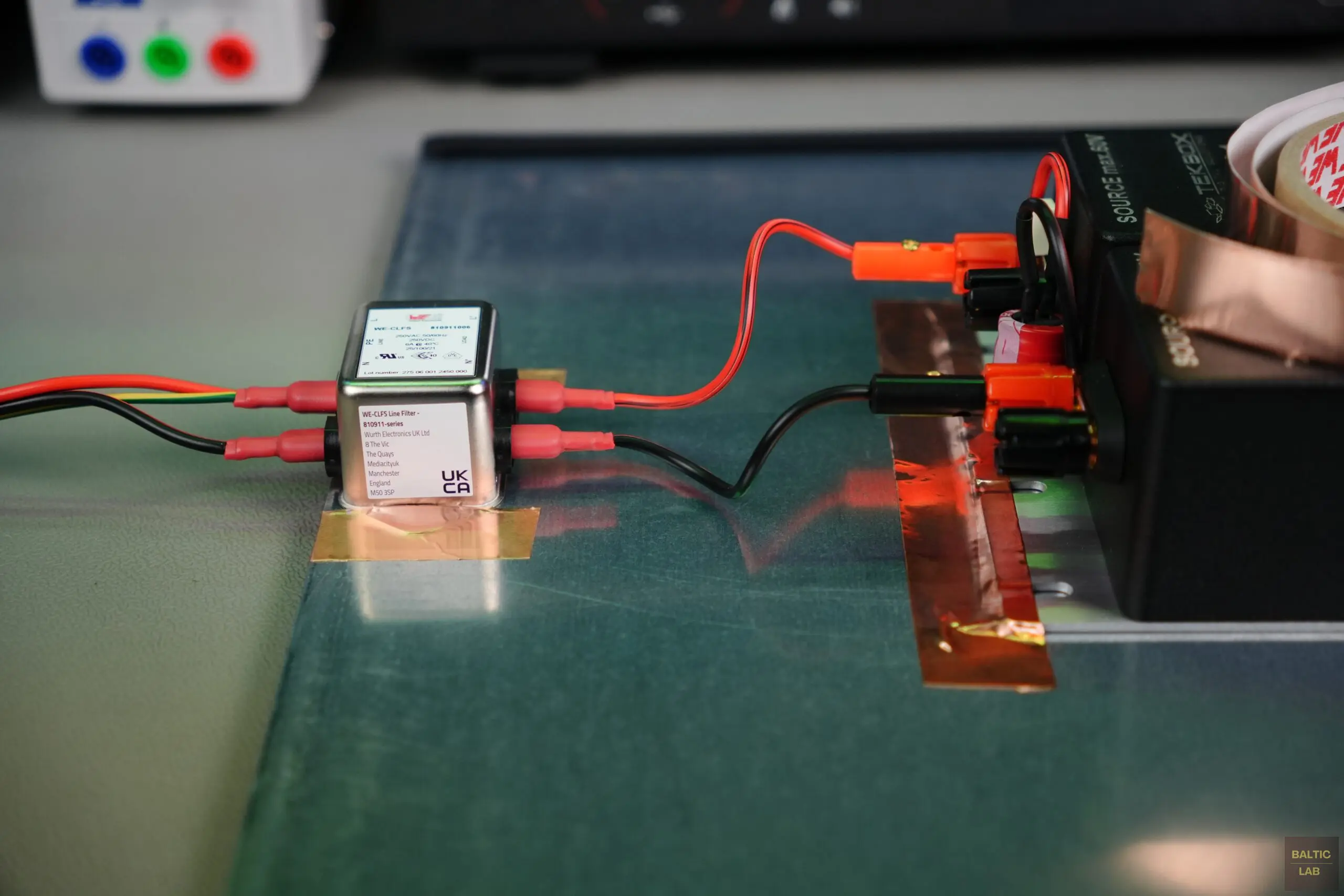
Figure 13: Supply voltage input section showing the line filter (left) and connections to the LISNs
For stricter limits, a 7 Ah sealed lead-acid battery is used. In this case, care must be taken to maintain the nominal supply voltage within the ±10 % tolerance as the battery discharges during measurement. A practical interim solution is to operate the battery in parallel with the power supply. The battery’s inherently low impedance provides effective suppression of residual power-supply noise. A fuse should be inserted in series with the battery to prevent damage to the LISNs in the event of an accidental short.
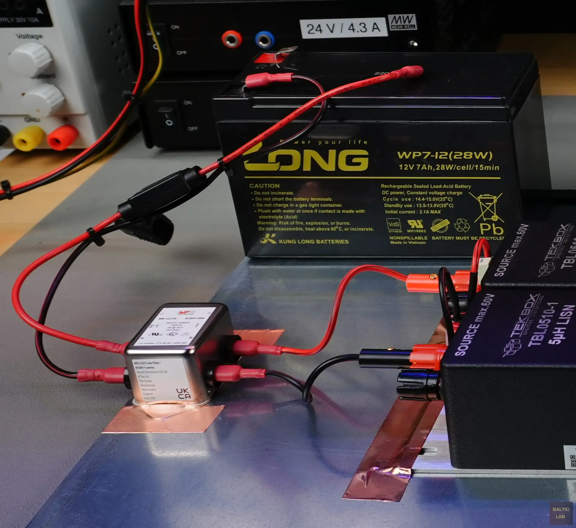
Figure 14: Sealed lead-acid battery with in-line fuse used as an alternative low-noise power supply source
Measurement Receiver & Software
The measuring instrument, including FFT-based receivers, must comply with the requirements of CISPR 16-1-1 [1]. The exact requirements could, and likely will, be the topic of a separate, more detailed article. Spectrum analyzers and scanning receivers are particularly useful for conducted emissions measurements. The peak detection performed by these instruments always produces a reading that is equal to or higher than the quasi-peak reading for the same bandwidth [2]. Correctly using spectrum analysers for EMC pre-compliance tests is quite involved [5]. For readers interested in the specifics of using a common low-cost spectrum analyzer, I recommend the excellent application note by TekBox. There is no need to reinvent the wheel here.
| Frequency Range | CISPR Filter Bandwidth |
|---|---|
| 9 kHz – 150 kHz | 200 Hz |
| 150 kHz – 30 MHz | 9 kHz |
| 30 MHz – 1 GHz | 120 kHz |
| > 1 GHz | 1 MHz |
For my test setup, I am using a Rigol RSA5065N with the EMI measurement option [6], together with the TekBox EMCview PC software [7]. The EMI option provides the required CISPR resolution bandwidths (Table 2) and the standardized CISPR peak, quasi-peak, and average detectors, which are essential for accurate emissions measurements. The TekBox EMCview software integrates seamlessly with many low-cost spectrum analyzers, including entry-level models from Rigol and Siglent. EMCview streamlines standard-compliant measurements substantially. Once the appropriate segment files, limit lines, and correction files (including LISN and cable corrections) are loaded, the process is largely automated: start the scan, let it run, and wait for the results. Resolution bandwidths and detector settings are applied automatically in the background. The connection to the spectrum analyzer can be established conveniently via USB or Ethernet.
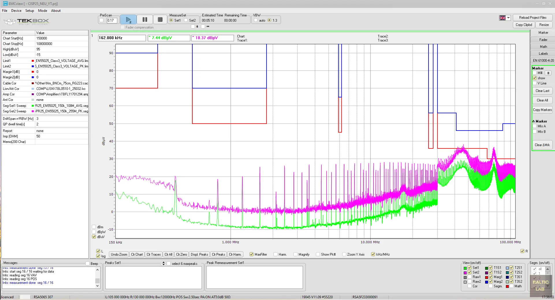
Figure 15: EMCview software configured with CISPR 25 Class 3 limits and correction factors for the LISNs, transient limiter, and BNC-to-N RG223 cable
Measurement
The conducted emissions on the supply lines are measured sequentially on the positive supply line and on the supply return line (ground) by connecting the spectrum analyzer to the measurement port of the corresponding LISN. The measurement port of any additional LISN inserted in the remaining supply line(s) must be terminated with a 50 Ω load [1, 2].
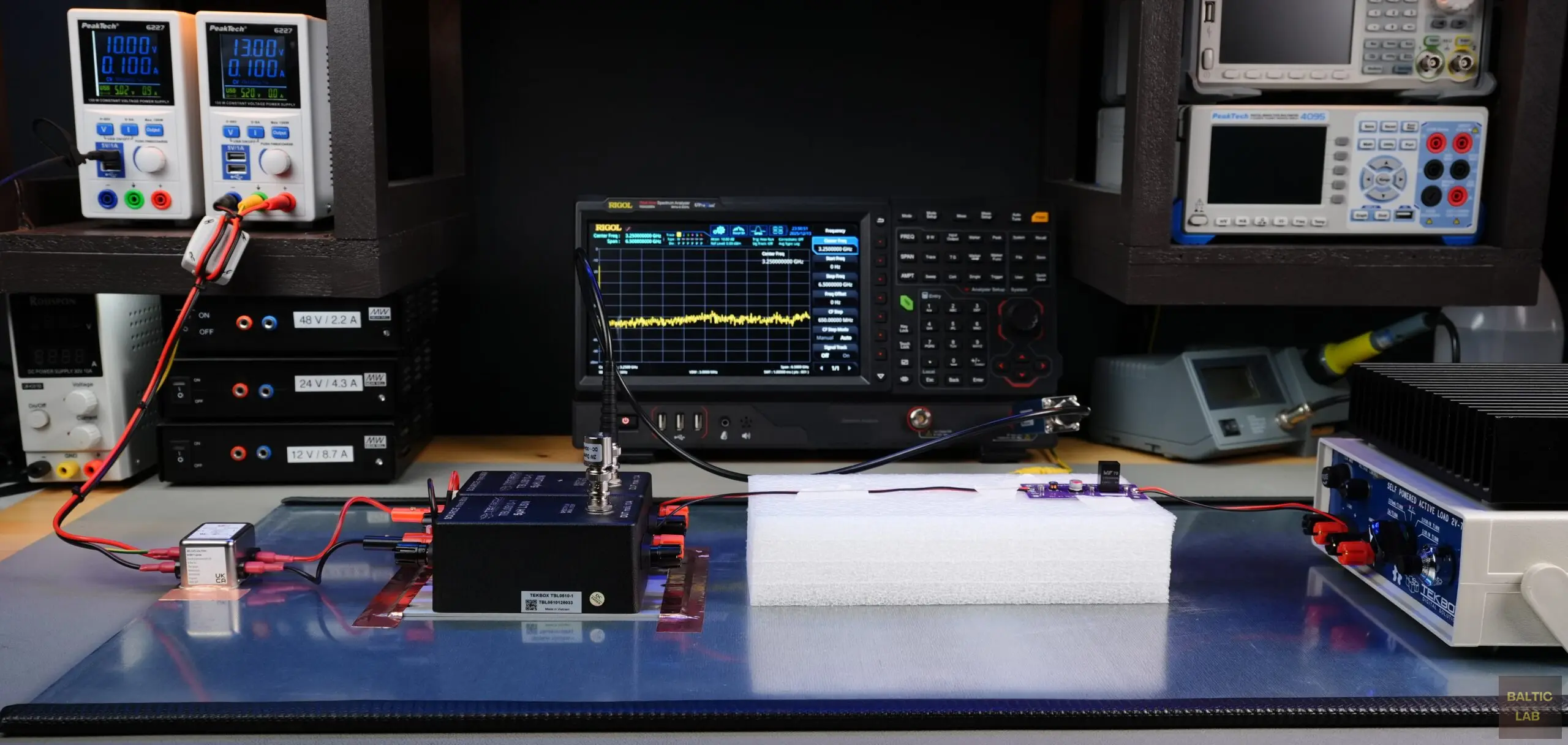
Figure 16: Complete CISPR 25 (voltage method) benchtop test setup
For a device to pass the test, it must not exceed any average or (quasi)-peak limit on either the supply line or the return line. A single limit exceedance at any frequency on any line is treated as a test failure.
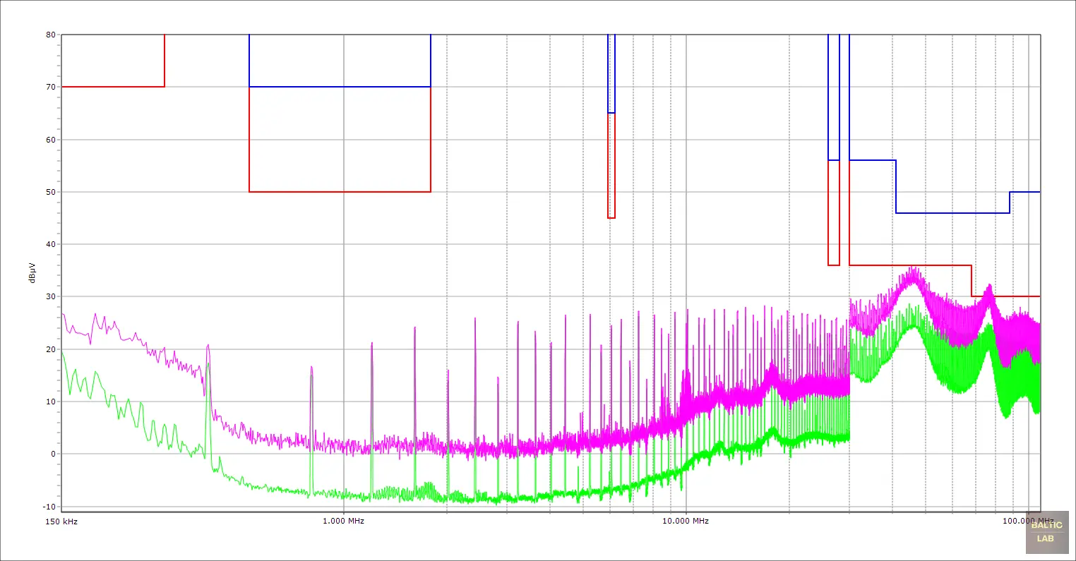
Figure 17: Conducted emissions measurement of a DUT with CISPR 25 Class 3 limits; peak (purple) and average (green) spectra shown alongside average limit (red) and peak limit (blue)
Side note: Although CISPR 25 defines limits for average, peak, and quasi-peak, (Tables 3 – 5) only the quasi-peak and average limits are legally binding for certification. Peak measurements are useful for quick pre-compliance screening or troubleshooting, but passing peak limits alone does not guarantee compliance. Accredited laboratories typically perform peak measurements for initial scans or debugging, but final certification always relies on quasi-peak and average measurements in accordance with the standard.
| Frequency Range (MHz) | Class 1 (dBµV) | Class 2 (dBµV) | Class 3 (dBµV) | Class 4 (dBµV) | Class 5 (dBµV) |
|---|---|---|---|---|---|
| 0.15 – 0.3 | 90 | 80 | 70 | 60 | 50 |
| 0.53 – 1.8 | 66 | 58 | 50 | 42 | 34 |
| 5.9 – 6.2 | 57 | 51 | 45 | 39 | 33 |
| 26 – 28 | 48 | 42 | 36 | 30 | 24 |
| 30 – 68 | 48 | 42 | 36 | 30 | 24 |
| 68 – 108 | 42 | 36 | 30 | 24 | 18 |
| Frequency Range (MHz) | Class 1 (dBµV) | Class 2 (dBµV) | Class 3 (dBµV) | Class 4 (dBµV) | Class 5 (dBµV) |
|---|---|---|---|---|---|
| 0.15 – 0.3 | 110 | 100 | 90 | 80 | 70 |
| 0.53 – 1.8 | 86 | 78 | 70 | 62 | 54 |
| 5.9 – 6.2 | 77 | 71 | 65 | 59 | 53 |
| 26 – 28 | 68 | 62 | 56 | 50 | 44 |
| 30 – 41 | 68 | 62 | 56 | 50 | 44 |
| 41 – 88 | 58 | 52 | 46 | 40 | 34 |
| 88 – 108 | 62 | 56 | 50 | 44 | 38 |
| Frequency Range (MHz) | Class 1 (dBµV) | Class 2 (dBµV) | Class 3 (dBµV) | Class 4 (dBµV) | Class 5 (dBµV) |
|---|---|---|---|---|---|
| 0.15 – 0.3 | 97 | 87 | 77 | 67 | 57 |
| 0.53 – 1.8 | 73 | 65 | 57 | 49 | 41 |
| 5.9 – 6.2 | 64 | 58 | 52 | 46 | 40 |
| 26 – 28 | 55 | 49 | 43 | 37 | 31 |
| 30 – 54 | 55 | 49 | 43 | 37 | 31 |
| 54 – 68 | 49 | 43 | 37 | 31 | 25 |
| 68 – 108 | 49 | 43 | 37 | 31 | 25 |
To ensure compliance with the standard, it is highly recommended to precede the actual measurement with a background scan performed with the complete setup in place but the device under test disabled or removed. This background scan verifies that noise from external sources (such as the power supply and environmental interference) remains at least 6 dB below all applicable limits.
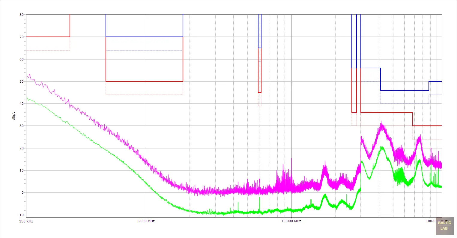
Figure 18: Background measurement evaluated against CISPR 25 Class 3 limits; grey traces below each limit indicate the required 6 dB margin
At the very least, the background scan allows you to distinguish DUT-generated emissions from external noise sources, even if the background itself exceeds the limits. In my laboratory setup, broadcast FM radio stations and certain LED room lights frequently couple into the test system within the VHF range, occasionally exceeding the limits on their own (Figs. 18 – 19). Which is one of the major disadvantages of not working inside a shielded room.
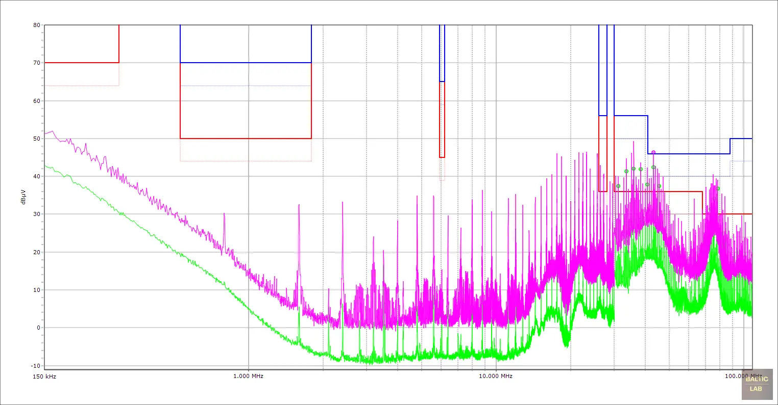
Figure 19: Background measurement with LED room lighting enabled, evaluated against CISPR 25 Class 3 limits; multiple limit exceedances observed above 30 MHz
Differential- and Common-Mode Separation
Let’s say your DUT fails the pre-compliance test, which happens more often than anyone would like. For effective troubleshooting, separating differential- and common-mode noise helps pinpoint the emission source and develop a suitable filtering strategy. While not specified in the standard, a dual-LISN setup facilitates measurement of individual noise components through straightforward addition or subtraction. Adding the noise signals from both LISNs in phase cancels the differential-mode component and yields the common-mode component at twice the amplitude of a single-line measurement. Conversely, subtracting the signals (or adding one with a 180° phase shift) cancels the common-mode component and leaves the differential-mode component, also doubled relative to a single-line measurement.
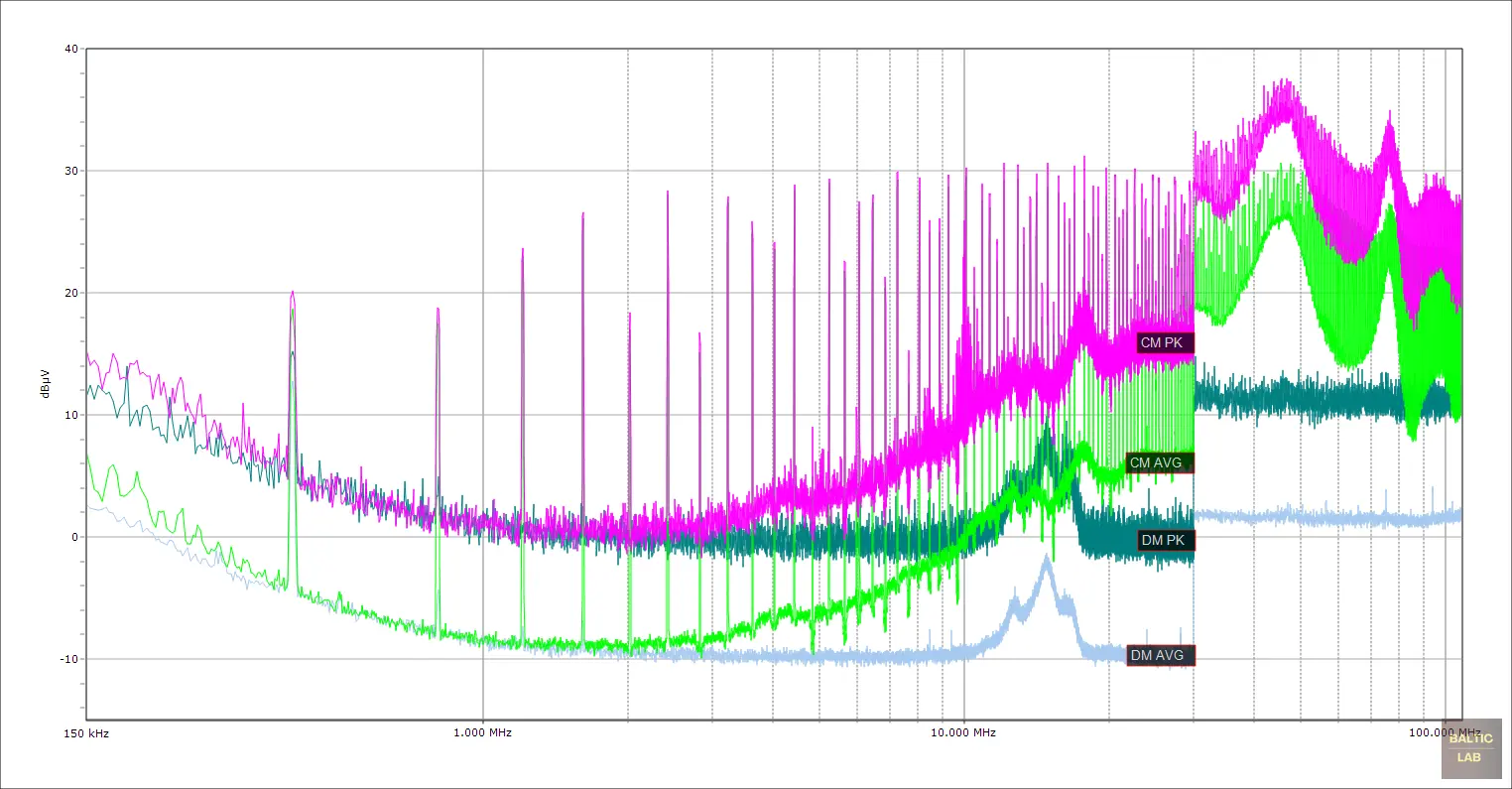
Figure 20: Conducted emissions measurement of a DUT with separated differential- and common-mode components, showing common-mode peak (CM PK), common-mode average (CM AVG), differential-mode peak (DM PK), and differential-mode average (DM AVG) spectra
Such addition or subtraction can be implemented directly using a modern oscilloscope’s math functions and FFT, with each LISN output connected to its own input channel. While this is useful for quick situational awareness, the oscilloscope’s FFT does not comply with the standard’s detector and sweep-time requirements, nor does it account for the frequency-dependent correction factors of the LISNs and test cables.
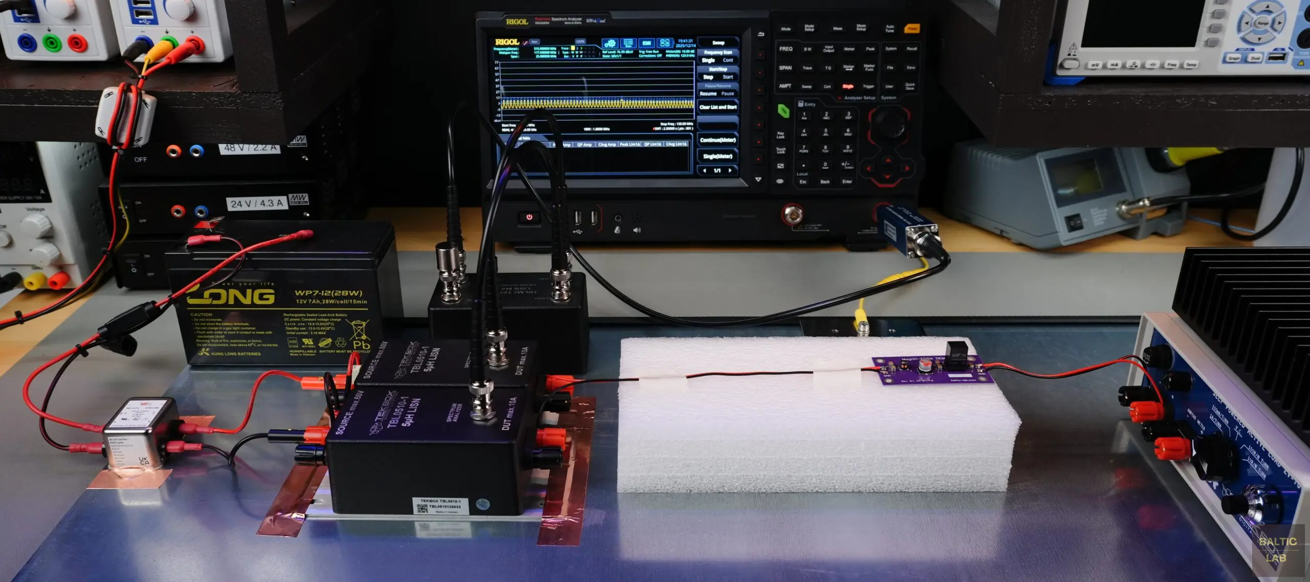
Figure 21: Modified test setup using a sealed lead-acid battery as a low-noise power source, with the LISN Mate installed for differential- and common-mode separation
For reliable differential- and common-mode measurements that can be used directly for line-filter design, a properly characterized combiner paired with a measurement receiver or spectrum analyzer should be used. In my setup, the TekBox TBLM2 LISN Mate is used [11]. It provides calibrated correction factors from 9 kHz to 110 MHz and functions as a dedicated common-mode/differential-mode separator. The LISN Mate connects to the outputs of both LISNs, and the isolated differential or common-mode component can then be taken from its respective output.
Optional Improvement: Shielded Tent
As outlined earlier, the standard requires measurements to be performed inside either a shielded enclosure (Faraday cage) or an absorber-lined shielded enclosure (ALSE). Implementing such an environment would defeat the purpose of this article, which focuses on a genuinely low-cost benchtop solution, although, in principle, a bench can certainly be placed inside a shielded enclosure. As a practical compromise, shielding tents made from conductive fabric are worth mentioning as a viable way to reduce external RF interference without the cost or complexity of a full chamber.

Figure 22: Shielded tent made from conductive fabric and aluminium profiles, showing the base plate with installed power-supply line filters and partially visible N- and BNC-type connectors
Due to space constraints, the shielding tent used here – a TekBox TBST measuring 86 cm × 48 cm × 48 cm – fits conveniently on a standard lab bench while providing sufficient shielding to suppress external interference during measurements [12]. It is, however, not large enough to accommodate the minimum required ground-plane size of 100 cm × 40 cm. The deviation is not standard-compliant but remains fairly insignificant and more than sufficient for my needs. Larger versions are available, up to 204 × 104 × 100 cm, but they currently exceed the remaining lab space. For that reason, this serves only as an honorable mention at the end of this article.
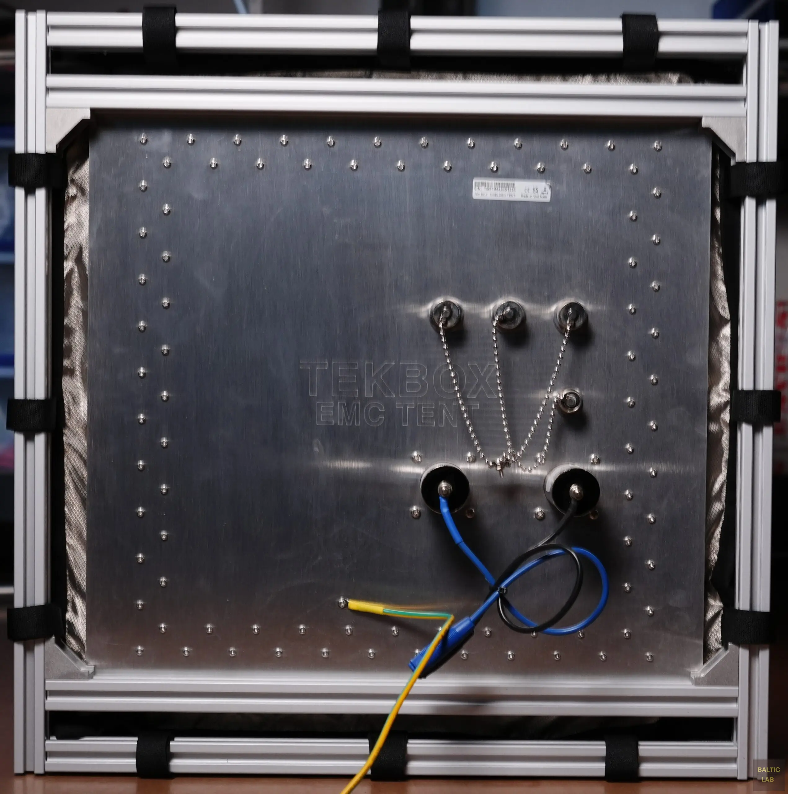
Figure 23: Base plate of the shielded enclosure showing N- and BNC-type connectors and the integrated supply line filters
Video
If a picture is worth a thousand words, a video is worth a million:
Conclusion
This article has shown that CISPR 25 conducted-emissions measurements can be carried out reliably on a standard lab bench using the voltage method. With disciplined grounding, controlled supply routing, and a correctly configured LISN to receiver chain, the approach delivers repeatable data. While it cannot substitute accredited compliance testing, it provides a practical and cost-effective way to uncover issues early, validate design changes, and build EMC confidence long before entering a certified lab.
Links and Sources:
[1] IEC, CISPR25: Vehicles, boats and internal combustion engines – Radio disturbance characteristics – Limits and methods of measurement for the protection of on-board receivers, 5th ed., IEC Std. 64645, Dec. 2021.
[2] DIN, DIN EN IEC 55025:2023-11 – Fahrzeuge, Boote und von Verbrennungsmotoren angetriebene Geräte – Funkstöreigenschaften – Grenzwerte und Messverfahren für den Schutz von an Bord befindlichen Empfängern (CISPR 25:2021), VDE 0879-2:2023-11, Nov.2023
[3] TekBox, “5 µH Line Impedance Stabilisation Network” [Online]. Available: https://www.tekbox.com/product/TBL0510-1_Manual.pdf.
[4] TekBox, “TBL0510-1 5UH Line Impedance Stabilisation Network LISN” [Online]. Available: https://www.tekbox.com/product/tbl0510-1-5uh-line-impedance-stabilisation-network-lisn/.
[5] TekBox, “How to correctly use spectrum analyzers for EMC pre-compliance tests” Apr. 2022, [Online]. Available: https://www.tekbox.com/product/AN_spectrum_analyzers_for_EMC_testing.pdf.
[6] Rigol, “RSA5065N” [Online]. Available: https://rigolshop.eu/products/spectrum-analyzers-rsa5000-rsa5065n.html.
[7] TekBox, “EMCview PC software for EMC pre-compliance testing” [Online]. Available: https://www.tekbox.com/product/emcview-pc-software-emc-compliance-testing/.
[8] Würth Elektronik, “WE-CLFS Line Filter | Passive Components | Würth Elektronik Product Catalog” [Online]. Available: https://www.we-online.com/en/components/products/WE-CLFS#810911006.
[9] Würth Elektronik, “WE-STAR-TEC | Passive Components | Würth Elektronik Product Catalog” [Online]. Available: https://www.we-online.com/en/components/products/WE-STAR-TEC#74271222.
[10] TekBox, “TBOH02 Self Powered Active Load” [Online]. Available: https://www.tekbox.com/product/tboh02-self-powered-active-load/.
[11] TekBox, “TBLM2 LISN Mate” [Online]. Available: https://www.tekbox.com/product/tblm2-lisn-mate/.
[12] TekBox, “TBST Shielded Tents” [Online]. Available: https://www.tekbox.com/product/tbst-shielded-tents/.
[13] Würth Elektronik, “WCAP-ATG8 | Passive Components | Würth Elektronik Product Catalog” [Online]. Available: https://www.we-online.com/en/components/products/WCAP-ATG8#860010780024.
[14] IEC, “Specification for radio disturbance and immunity measuring apparatus and methods – Part 1‑1: Radio disturbance and immunity measuring apparatus – Measuring apparatus,” CISPR 16‑1‑1, 5th ed., May 2019.
Westerhold, S. (2025), "Conducted Emissions on the Bench: Implementing the CISPR 25 Voltage Method". Baltic Lab High Frequency Projects Blog. ISSN (Online): 2751-8140., https://baltic-lab.com/2025/12/conducted-emissions-on-the-bench-implementing-the-cispr-25-voltage-method/, (accessed: March 1, 2026).

- Conducted Emissions on the Bench: Implementing the CISPR 25 Voltage Method - December 15, 2025
- WebP-Images without Plugin - January 14, 2025
- Firewall Rules with (dynamic) DNS Hostname - January 14, 2025
jsmes osburn
I’m an EMC professional based in Berlin, currently working on an open-source EMC software project.
I’ve also been developing a simulator for VXI-11 instrumentation, mainly to support testing and automation workflows.
I’ve been following your work at Baltic-Lab and thought it might be of interest to connect.
Best regards,
james osburn
EMC Engineer
Are you testing a ignition system component, or why you are using the 1000µF capacity?
Where can I find the information about the missing capacity in the GND-LISN? I do not find any information in the CISPR25:2022 or older ones.
Sebastian Westerhold
While the 1000 µF capacitor is only required for testing components that are part of the ignition system, it does no harm if it is also fitted for other tests.
The absence of an input capacitor on the GND LISN is obvious from the standard itself: both the positive and negative supply terminals of the GND LISN are connected to the reference ground plane and the negative supply wire. In other words, they are shorted together, so any capacitor would be shorted as well. You may leave it in place physically, but electrically it does not exist. Not everything is spelled out explicitly in standards. Most of them assume a certain level of critical thinking as a prerequisite. I agree this is a rather daring approach to assume most people are capable of thinking on their own, but it is what it is.