DIY Spark Gap Transmitter

This article plunges you into the mesmerrizing world of early radio technology through the assembly and analysis of a DIY spark gap transmitter. This project offers a practical insight into the fascinating dynamics of damped harmonic oscillators and explains charasteristics such the logarithmic decrement, decay rate, damping factor, q factor, and beyond. Prepare to spark your curiosity in a technology that once revolutionized global communication.

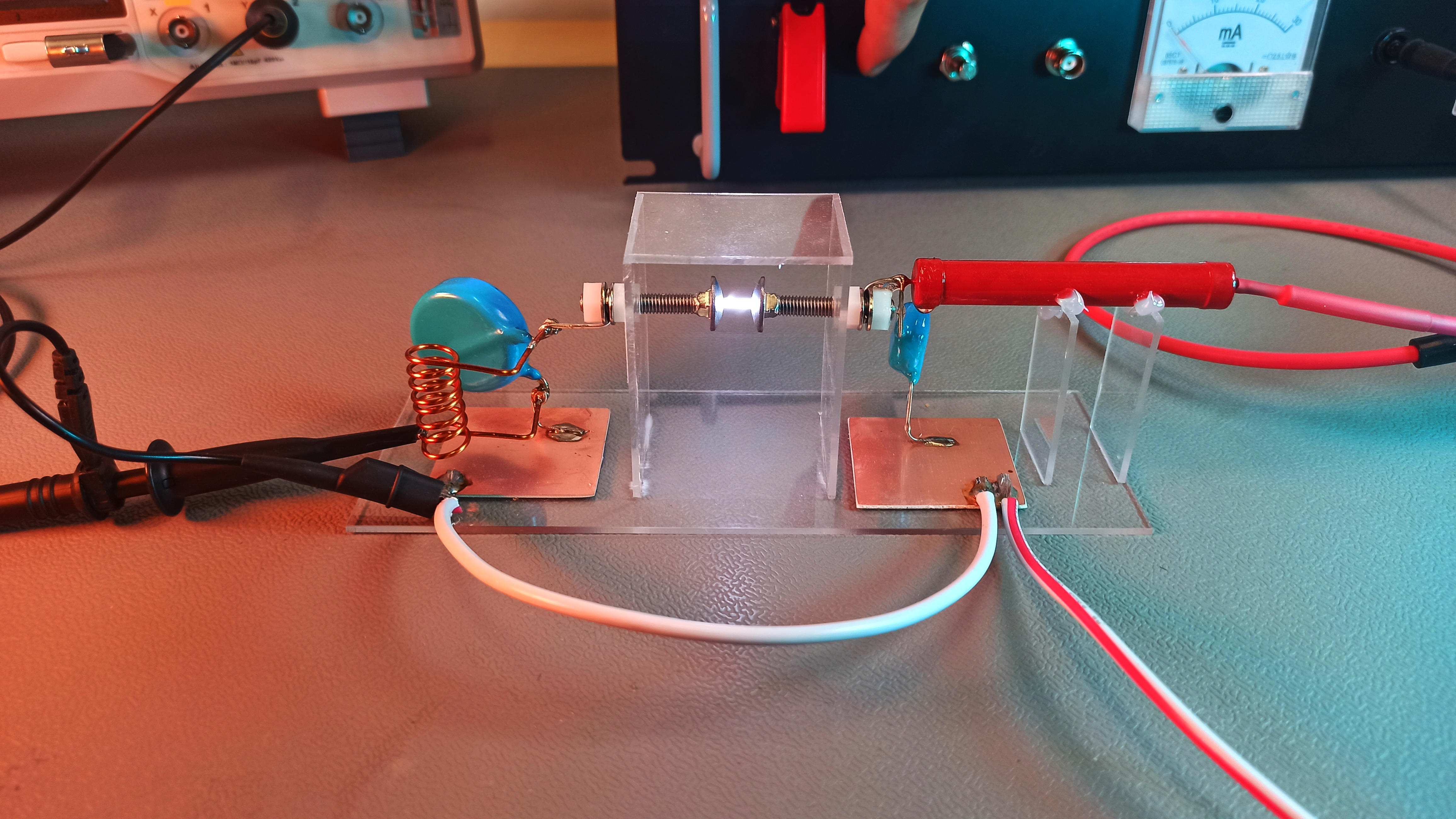
Simple spark gap transmitter built from a handful of components on a acrylic glass base

Circuit

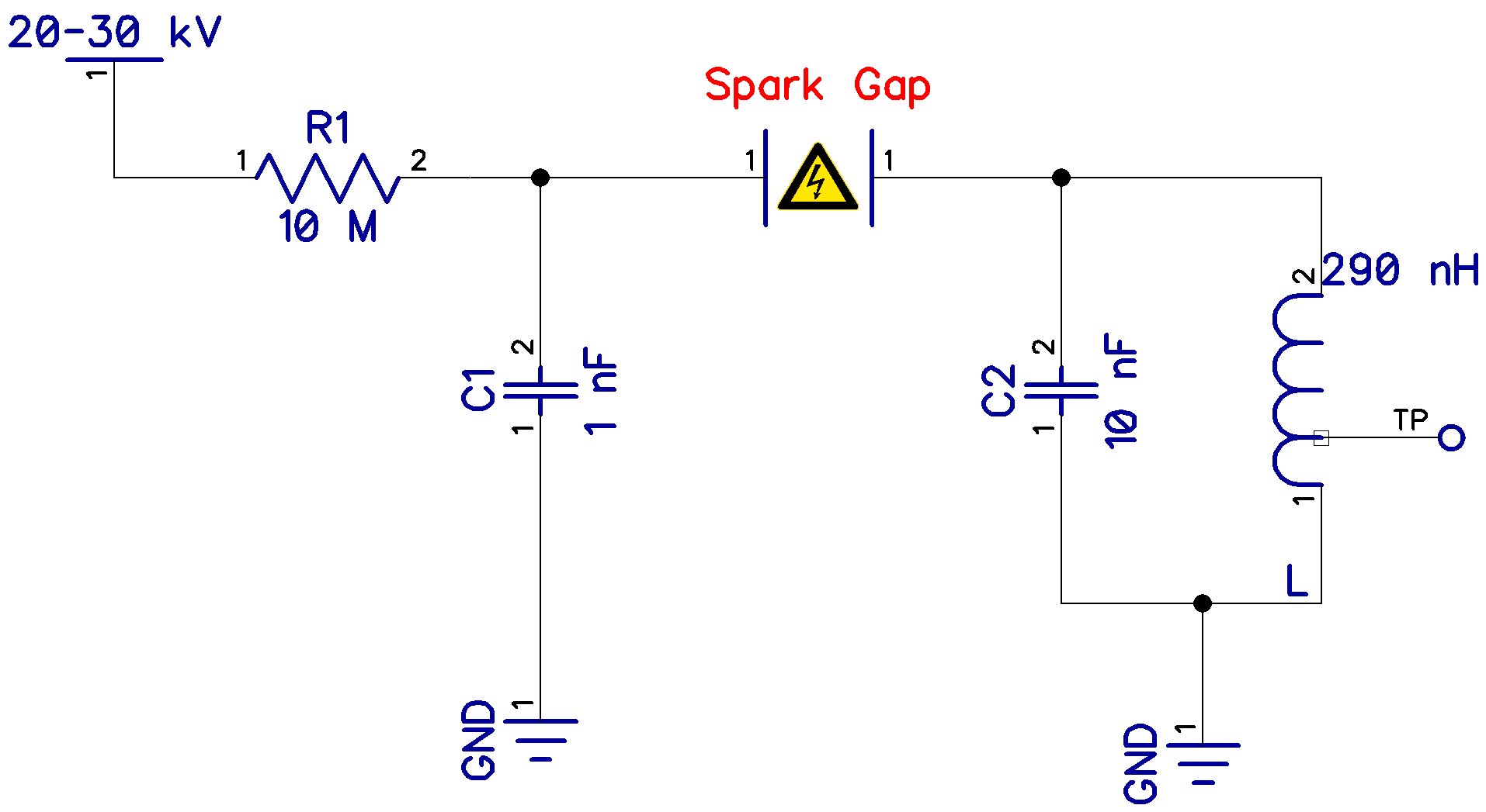
The circuitry in a spark gap transmitter is fairly straightforward. It’s worth noting, however, that the spark gap transmitters from the Titanic era were constructed differently. Nonetheless, the underlying principle is unchanged, and my design is primarily crafted for display purposes.

Simple spark gap transmitter with an emission frequency of around 3 MHz.

The spark gap is constructed using carriage bolts and acrylic. The breakdwon voltage of air is around 3 kV/mm. At least when assuming an idealized homogeneous field and an electrode spacing of 10mm. While this simplification ignores a bit of reality, delving into Paschen’s law is beyond the scope of this article. The spark gap is set for a breakdown voltage of roughly 18 kV, equivalent to an electrode gap of approximately 6mm.

The breakdown voltage is reached at a rate determined by R1 and C1, as outlined in Equation 1. Where V_C1 is the voltage across C1, V_in the supply voltage of the circuit and t represents time in seconds. Specifically, the voltage across C1 approximates 63% of the input voltage after one time constant (equal to R1 multiplied by C1). This percentage climbs to roughly 87% after two time constants. Thus, by varying the input voltage, this RC circuit facilitates a straightforward method for modifying the spark gap’s triggering frequency.

(1) $\begin{equation*} V_{C1} = V_{in} (1 - e^{\frac{-t}{R_1 C_1}}) \end{equation*}$

Once the breakthrough voltage is reached, the spark gap activates, creating an almost direct path for electron flow. Subsequently, charge balancing among C1, C2, and L2 energizes the resonant LC circuit formed by C2 and L1. The resonant frequency mainly depends on L1 and C2 (Eq. 2). This statement is generally accurate, though certain factors can partially invalidate this assumption. These factors will be discussed in detail when presenting the actual test results. The components values used in this example should yield a resonant frequency of close to 3 MHz (Eq. 3).

(2) $\begin{equation*} f_r = \frac{1}{2 \pi \sqrt{LC}} \end{equation*}$

(3) $\begin{equation*} f_r = \frac{1}{2 \pi \sqrt{290\;nH \cdot 10\;nF}} = 2.95543\;MHz \end{equation*}$

The components in this circuit must be rated for the high voltage applied in this experiment. R1, C1, and C2 can withstand voltages exceeding 30 kV. L1 is a handmade, 8-turn air core inductor wound from enamelled copper wire, featuring a tap 1.5 windings from the ground connection to connect an antenna or oscilloscope probe. This tap also facilitates basic impedance matching for connecting a 50-ohm antenna to the circuit. For readers in the U.S., it’s important to note that the Federal Communications Commission (FCC) strictly prohibits damped wave emissions altogether. The reasons behind the term “damped wave emissions” and why regulatory authorities might disapprove will soon become clear when the emissions from this circuit are examined closer.

Testing and Analysis

For the initial test, a length of wire is soldered directly to the inductor’s tap. The input of the circuit is connected to my DIY high-voltage power supply. An XHDATA D-808 multi-band receiver, set to 2.995 MHz and Amplitude Modulation (AM), is utilized to monitor the emissions while keying the high-voltage supply on and off. The sound produced is clearly audible and difficult to characterize. Adjusting the supply voltage varies the spark gap’s firing rate, which in turn modifies the pitch of the audio.

The demodulated audio was recorded twice: first utilizing the SDRplay RSPdx and SDRuno and then with the XHDATA D-808 feeding directly into my sound card:

Next, the antena wire is removed and an oscilloscope is connected. Since I was not really in the mood of potentially frying one of my better scopes, I used the scope where high voltage induced damage would upset me the least. So I apologize in advance for the moderate to bad screen captures. With the oscilloscope set to single capture, the spark gap is fired and the resulting output signal recorded.

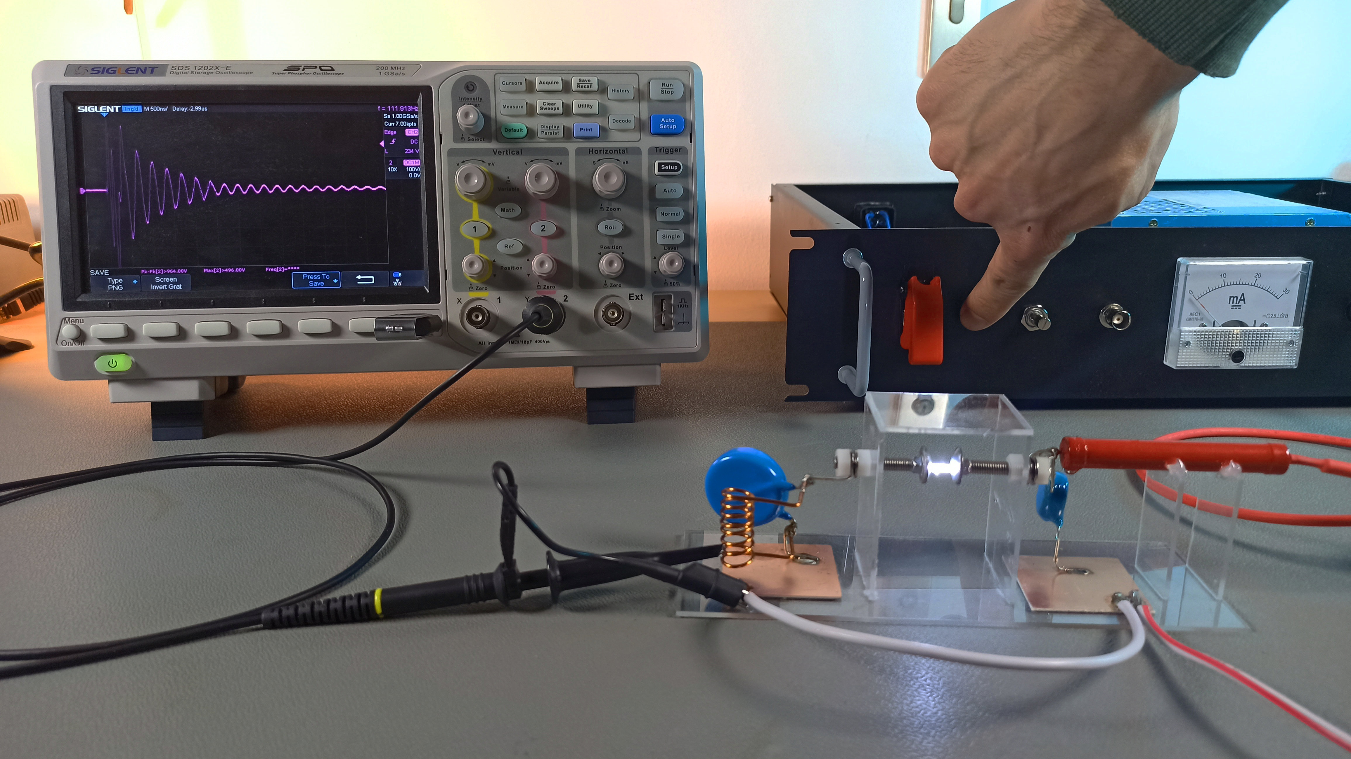
Test setup: High-voltage power supply (right), DIY spark gap transmitter (center) and oscilloscope (left)

A sinusoidal signal, characterized by a rapidly decaying amplitude, becomes immediately noticeable. The frequency is roughly 3 MHz. Observant readers may also detect approximately 1.5 cycles of a signal at a different frequency preceding the 3 MHz This off-frequency component will be ignored for now and addressed later in this article. It should be noted that this pulse repeats everytime the spark gap is triggered.

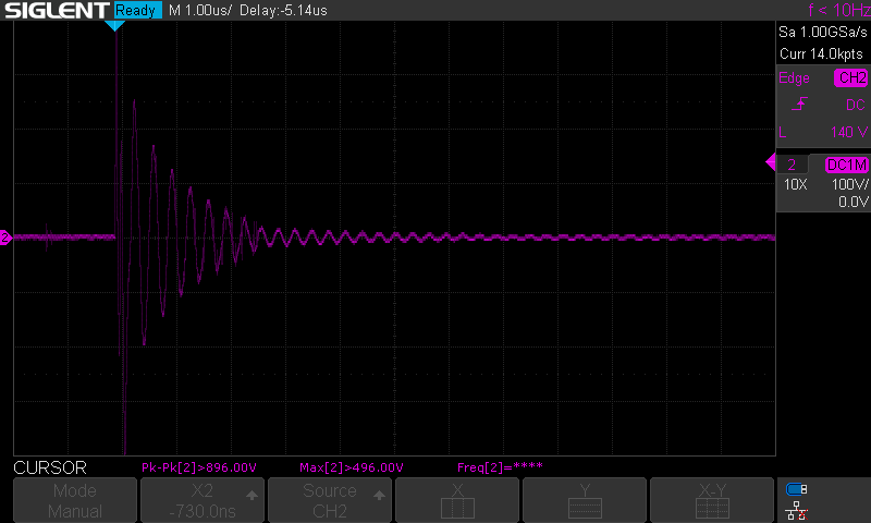
Waveform of a single emission pulse from the spark gap transmitter.

Observing that the amplitude envelope exhibits an exponential decay requires little creativity, showcasing a typical characteristic of damped oscillations. This behavior aligns with the principles of a damped harmonic oscillator, a common phenomenon in physics regardless of the system—be it an LC circuit, a spring, or a pendulum. As such, the output signal follows the behaviour shown in equation 4. Where V(t) is the output voltage at the time t, A the initial Amplitude, $\delta$ the decay rate, $\omega$ the angular frequency ( $2 \pi f$ ). Characterizing all of those parameters isn’t all too difficult.

(4) $\begin{equation*} V(t) = A e^{- \delta t} \cos(\omega t) \end{equation*}$

Closeup of a single output pulse from the spark gap transmitter

With proper markers in place and zoomed in a bit, and still ignoring the first 1.5 cycles, the frequency can be confirmed to be around 3 MHz, 2.976 MHz to be precise. The amplitude of the first peak is 266 V, the second peak is at 174 V and the consequent 3 peaks are at 126 V, 96 V, 72 V and 52 V. This is all the information needed to calculate the so called logarithmic decrement (Eq. 5 and 6).

(5) $\begin{equation*} \Lambda = \frac{1}{n} \ln(\frac{A}{A_n}) \end{equation*}$

(6) $\begin{equation*} \Lambda = \frac{1}{6} \ln(\frac{266\;V}{52\;V}) \approx 0.272 \end{equation*}$

Relating the logarithmic decrement to the time period of the oscillation (1/f), immediately yields the decay rate $\delta$ (Eq. 7 and 8).

(7) $\begin{equation*} \delta = \frac{\Lambda}{T_d} \end{equation*}$

(8) $\begin{equation*} \delta = \frac{0.272}{3.36\; \cdot 10^{-7}} \approx 8.1 \cdot 10^5 \end{equation*}$

With some basic math out of the way, the damped wave output of the spark gap transmitter can now mathematically be expressed as a function of time (Eq. 9).

(9) $\begin{equation*} V(t) = 266\;V\;e^{-8.1 \cdot 10^5\;t} \cos(2\;\pi\;2.976\cdot 10^6\;t) \end{equation*}$

This derived equation is then plotted using Python. The result looks indeed a lot like the signal captured with the oscilloscope.

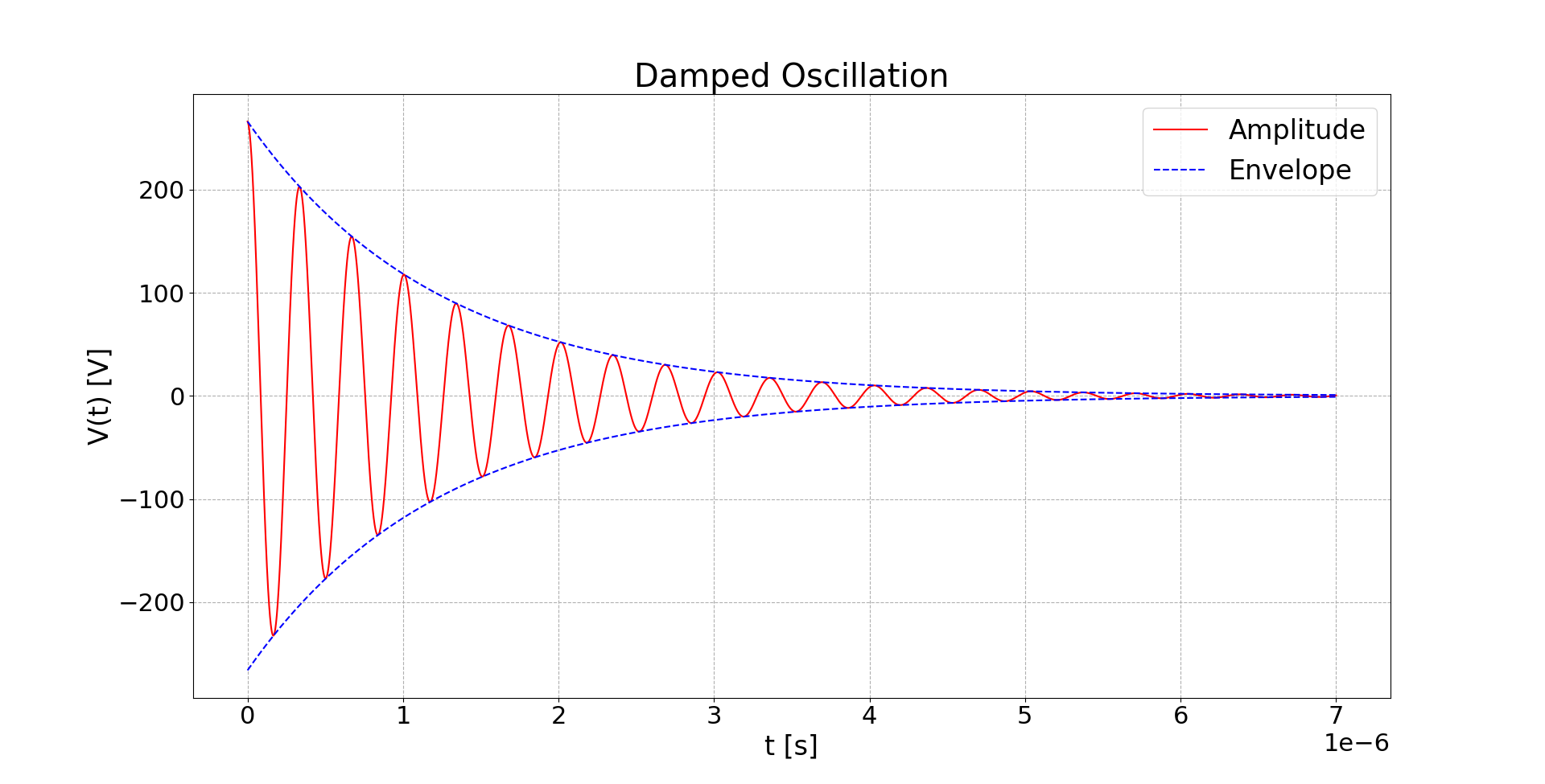
Plot of a single output pulse with the parameters previously calculated

One thing that is missing from the plot, however, is the faster oscillation at the beginning, that I elected to ignore for now. Upon further inspection, this undesired oscillation occurs at around 10.42 MHz.

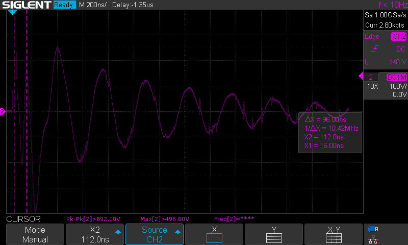
10.42 MHz oscillation at the beginning of each output pulse.

10.42 MHz is close enough to 3.33 times higher than the desired resonant frequency. Assuming that the inductance of L1 is constant, rearranging Equation 2 would yield such an oscillation if the parallel capacitance is around 1 nF. Which coincidentally is the capacitance of C1. The problem is that the moment the spark gap is triggered, C1 is fully charged and C2 is empty. Initially, the fully charged C1 alone interacts with L1, with C2’s contribution delayed, a process taking about 96 ns. This isn’t the sole issue. Once the spark gap triggers, incorporating both capacitors alters the resonant frequency, creating a third frequency slightly below that of C1 and L1 in isolation. The desired resonant frequency, determined solely by C1 and L1, is only achieved post spark extinguishment. Ignoring parasitics of course. Accordingly, the output spectrum looks fairly unappealing.

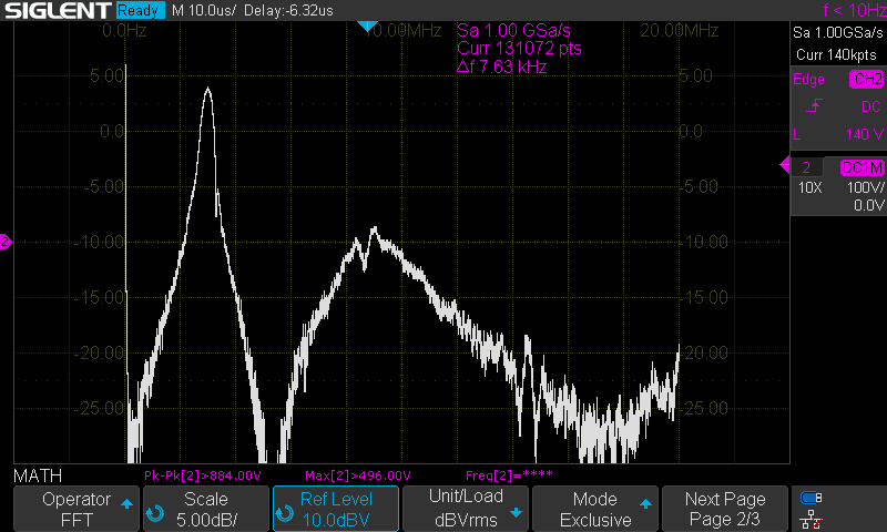
Output spectrum of the spark gap transmitter.

The output spectrum looks like an electromagnetic interference nightmare. Which answers the question of why regulatory agencies might have an issue with such transmitters. Speaking of bandwidth, since $\Lambda$ has been previously calculated, it’s just a small step to calculate the quality factor Q of this shocking harmonic oscillator. The first step is to calculate the damping ratio $\zeta$ from $\Lambda$ (Eq. 10) through which the quality factor Q can be calculated using Equation 12.

(10) $\begin{equation*} \zeta = \frac{\Lambda}{\sqrt{(2 \pi)^2 + \Lambda^2}} \end{equation*}$

(11) $\begin{equation*} \zeta = \frac{0.272}{\sqrt{(2 \pi)^2 + 0.272^2}} \approx 0.04324 \end{equation*}$

(12) $\begin{equation*} Q = \frac{1}{2 \zeta} \end{equation*}$

(13) $\begin{equation*} Q = \frac{1}{2\cdot0.04324} \approx 11.56 \end{equation*}$

Plugging all the values into the Equations yields a numerical Q factor of 11.56 (Eq. 10 and 13). At a frequency of 3 MHz this corresponds to a half-power bandwidth of approximately 260 kHz. Which seems to align reasonably well enough with the FFT spectrum.

Video

If a picture is worth a thousand words, then a video is worth a million. Therefore, I took the time and effort to also post a video on my YouTube channel:

Conclusions

Links and Sources:

[1] “DIY: Adjustable 30 kV High Voltage Power Supply”, Baltic Lab: https://baltic-lab.com/

Please cite this article as:
Westerhold, S. (2024), "DIY Spark Gap Transmitter". Baltic Lab High Frequency Projects Blog. ISSN (Online): 2751-8140., https://baltic-lab.com/2024/04/diy-spark-gap-transmitter/, (accessed: April 29, 2024).

Funding:

If you liked this content, please consider contributing. Any help is greatly appreciated.

One thought on “DIY Spark Gap Transmitter”


Lima on April 9, 2024 at 6:28 am said:

Nice analysis! The interaction of the 1nF capacitor is something i intuitively already was wondering about, but never actually have seen in an analysis.
I do see a limitation in your test: the lack of a simulated antenna system.
Books from the late 1910s, early 1910s show that the overall bandwidth of a Wien bridge quenched spark transmitter operating on the 500khz maritime band, can be narrower than 50kHz IIRC (-6 or -12dB points, i need to dig up the actual books to make sure i got the right numbers). Yes, really that narrow.
This is very dependent on the characteristics of the antenna used. The antenna and antenna coil together form a resonant circuit too. Care must be taken that the coupling between the primary and secondary coils is not too tight to avoid the typical double hump curve of an overcritically coupled band filter. Different degrees of coupling need to be used for simple ball gap transmitters, and the more sophisticated Wien quenched gap transmitters. One must be coupled as loosely as possible, the other must be coupled much stronger but i have forgotten which one’s which. Even back in the day, the books report on how hard it was to get them absolutely dialed in, and operating quietly without interference.
The spark gap itself needs to be quenched as soon as possible to avoid losses (and therefore a lowering of the Q) due to the partially ionized path. My personal experience is that zinc plated steel hardware is very bad for this. Brass spheres are already better and about the best you can get as a casual experimenter, without getting into the Wien bridge territory with extremely smooth machined surfaces that need to be 0,1 to 0,2mm apart.

Building a noisy spark gap transmitter is easy. Doing it according to the dark arts of the 1910s is a whole different beast. They can be cleaned up significantly, but you need extensive knowledge about it.